When you want to pull information from a table, the Excel VLOOKUP function is a typical solution. Its
ability to dynamically lookup and retrieve information from a table is a
game-changer for many users, so you'll find it everywhere.
And yet, although VLOOKUP is a relatively easy to use, there is plenty that can go wrong. One reason is that VLOOKUP has a major design flaw — by default, it assumes you're OK with an approximate match. Which you probably aren't.
This can cause results that look completely normal, even though they are totally incorrect. Trust me, this is NOT something you want to try to explain to your boss, after she's already sent your spreadsheet to management :)
Read below learn how to manage this challenge, and discover other tips for mastering the Excel VLOOKUP function.
If you have a well structured table, with information arranged vertically, and a column on the left which you can use to match a row, you can probably use VLOOKUP.
VLOOKUP requires that the table be structured so that lookup values appear in the left-most column. The data you want to retrieve (result values) can appear in any column to the right. When you use VLOOKUP, imagine that every column in the table is numbered, starting from the left. To get a value from a particular column, simply supply the appropriate number as the "column index". In the example below, we want to look up the email address, so we are using the number 4 for column index:

In the above table, the employee IDs are in column 1 on the left and the email addresses are in column 4 to the right.
To use VLOOKUP, you supply 4 pieces of information, or "arguments":
This means that VLOOKUP can only get data from columns to the right of first column in the table. When lookup values appear in the first (leftmost) column, this limitation doesn't mean much, since all other columns are already to the right. However, if the lookup column appears inside the table somewhere, you'll only be able to lookup values from columns to the right of that column. You'll also have to supply a smaller table to VLOOKUP that starts with the lookup column.

You can overcome this limitation by using INDEX and MATCH instead of VLOOKUP.


The formula in H6 to lookup year based on an exact match of movie title is:
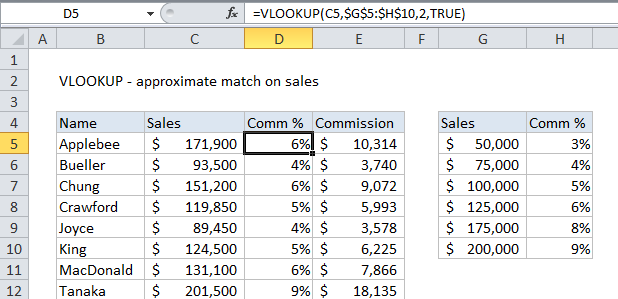
The formula in D5 does an approximate match to retrieve the correct commission:
For exact match, use FALSE or 0. For approximate match, set range_lookup to TRUE or 1:
This is a dangerous default because many people unwittingly leave VLOOKUP in it's default mode, which can cause an incorrect result when the table is not sorted.
To avoid this problem, make sure to use FALSE or zero as the 4th argument when you want an exact match.
Video: How to use VLOOKUP for approximate matches
Felienne Hermans has a great example of this problem here, from a cool analysis she did on actual Enron spreadsheets!

Because the customer id exists in both tables, you can use this value to pull in the data you want with VLOOKUP. Just configure VLOOKUP to use the id value in table one, and the data in table 2, with the required column index. In the example below, we are using two VLOOKUP formulas. One to pull in the customer name, and the other to pull in the customer state.

A classic example is grades, where you need to assign a grade based on a score:

In this case, VLOOKUP is configured for approximate match, so it's important that the table be sorted in ascending order.
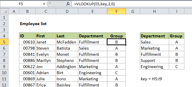
But you can also use VLOOKUP to assign arbitrary categories. In the example below, we are using VLOOKUP to to calculate a group for each department using a small table (named "key") that defines the grouping.
For example, because the lookup value and table array are absolute, we can copy the formula across the columns, then come back and change the column index as needed.

For example, in the employee data example above, you can name the input cell "id" and then name the data in the table "data", you can write your formula as follows:

Not only is this formula easier to read, but it's also more portable, since named ranges are automatically absolute.
In this example, the lookups for Rank and Sales were broken when a new column was inserted between Year and Rank. Year continues to work because it is on the left of the inserted column:

To avoid this problem, you can calculate a column index as described in the next two tips.
For example, with the employee data below, we can use the COLUMN function to generate a dynamic column index. For the first formula in cell C3, COLUMN by itself will return 3 (because column C is third in the worksheet) so we simply need to subtract one, and copy the formula across:

All formulas are identical with no post-editing required.
The formula we are using is this:
This is sometimes called a two-way lookup since you are looking up both the row and the column.
An example would be looking up sales for a salesperson in a particular month, or looking up the price for a particular product from a particular supplier.
For example, suppose you have sales per month, broken out by salesperson:

VLOOKUP can easily find the sales person, but it has no way to handle the month name automatically. The trick is to to use the MATCH function in place of a static column index.

Notice that we give match a range that includes all columns in the table in order to "sync up" the the column numbers used by VLOOKUP.
Excel provides two wildcard characters: an asterisk (*) matches one or more characters, and a question mark (?) matches one character.
For example, you can type an asterisk directly into a cell and refer to it as a lookup value with VLOOKUP. In the screen below, we have entered "Mon*" into H3, which is a named range called "val". This causes VLOOKUP to match the name "Monet".
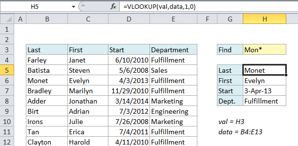
The formula in this case is simple:
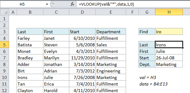
In this case, we are concatenating the asterisk to the lookup value inside the VLOOKUP function:
Once you start using VLOOKUP, you're bound to run into the #N/A error, which occurs when VLOOKUP isn't able to find a match.
This is a useful error, because VLOOKUP is telling you clearly that it can't find the lookup value. In this example, "Latte" doesn't exist as a beverage in the table, so VLOOKUP throws an #N/A error

The formula in this case is a completely standard exact match:
The easiest way to trap errors with VLOOKUP is to wrap VLOOKUP in the IFERROR function. IFERROR allows you to "catch" any error and return a result of your choosing.
To trap this error and display a "not found" message instead of the error, you can simply wrap the orignal formula inside of IFERROR and set the result you want:

If the lookup value is found, no error occurs and VLOOKUP function returns a normal result. Here is the formula:
In the following example, the ids for the planet table are numbers entered as text, which causes VLOOKUP to return an error since the lookup value is the number 3:

To solve this problem, you need to make sure the lookup value and the first column of the table are both the same data type (either both numbers or both text).
One way to do this is to convert the values in the lookup column to numbers. An easy way to do this is to add zero using paste special.
If you don't have easy control over the source table, you can also adjust the VLOOKUP formula to convert the lookup value to text by concatenating "" to the value like so:

If you can't be certain when you'll have numbers and when you'll have text, you can cater to both options by wrapping VLOOKUP in IFERROR and writing a formula to handle both cases:
For example, a common use of nested IFs is to assign grades based on a score of some kind. In the example below, you can see a formula has been build with nested IFs to do just that, using the grade key at the right as the guide.
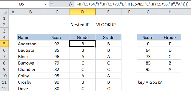
The full nested IF formula looks like this:
By contrast VLOOKUP can assign the same grades with a simple formula. All you need to do is make sure the grade key table is set up for VLOOKUP (i.e. it most be sorted by score, and contain brackets to handle all scores).
After defining a named range "key" for the grade key table, the VLOOKUP formula is very simple and generated the same grades as the original nested IFs formula:
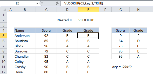
With the grade key table named "key" we have a very simple VLOOKUP formula:
Video: How to replace nested IFs with VLOOKUP
This means you can't easily do things like look up an employee with the last name of "Smith" in "Accounting", or look up an employee based on first and last names in separate columns.
However, there are ways overcome this limitation. One workaround is to create a helper column that concatenates values from different columns to create lookup values that behave like multiple conditions. For example, here we want find the department and group for an employee, but the first name and last name appear in separate columns. How can we lookup both at once?

First, add a helper column that simply concatenates first and last names together:

Then configure VLOOKUP to use a table that includes this new column, and join first and last names for the lookup value:

The final VLOOKUP formula looks up first and last names together using the helper column as the key:
The background: imagine that you have a lot of order data, say, more than 10,000 records and you are using VLOOKUP to lookup the order total based on the order id. So, you are using something like this:
The problem is that exact matches are really slow, because Excel must proceed in a linear fashion through all values until it finds a match or not.
Conversely, approximate matches are lightning fast because Excel is able to do what's called a binary search.
The problem with binary searches however (i.e. VLOOKUP in approximate match mode) is that VLOOKUP can return the wrong result when a value isn't found. Worse, the result might look completely normal, so it can be very difficult to spot.
The solution is to use VLOOKUP twice, both times in approximate match mode. The first instance simply checks that the value really exists. If so, another VLOOKUP is run (again, in approximate match mode) to fetch the data you want. If not, you can return any value you want to indicate that a result was not found.
The final formula looks like this:
Note: Your data must sorted to use this trick. It's simply a way to protect against a missing lookup value, while maintaining a fast lookup.
The gist is this: INDEX + MATCH can do everything that VLOOKUP (and HLOOKUP) can do, with more power, speed, and flexibility, at the cost of a bit more complexity. So, those in favor of INDEX + MATCH will argue (very sanely) that you might as well start off learning INDEX and MATCH, since it gives you a better toolset in the end.
The argument against INDEX + MATCH is that it requires two functions instead of one, so it is inherently more complex for users (especially new users) to learn and master.
My two cents is that if you use Excel frequently, you're going to want to learn how to use INDEX and MATCH. It's a very powerful combination.
But I also think you should learn VLOOKUP, which you'll run into everywhere, often in worksheets you inherit from others. In straightforward situations, VLOOKUP will get the job done just fine with no fuss.
https://www.deskbright.com/excel/how-to-do-a-vlookup/
Did I miss anything? Have questions? Feel free to leave a comment below.
This amazing article is written by my friend Dave Bruns from (exceljet.net)
And yet, although VLOOKUP is a relatively easy to use, there is plenty that can go wrong. One reason is that VLOOKUP has a major design flaw — by default, it assumes you're OK with an approximate match. Which you probably aren't.
This can cause results that look completely normal, even though they are totally incorrect. Trust me, this is NOT something you want to try to explain to your boss, after she's already sent your spreadsheet to management :)
Read below learn how to manage this challenge, and discover other tips for mastering the Excel VLOOKUP function.
1. How VLOOKUP works
VLOOKUP is a function to lookup up and retrieve data in a table. The "V" in VLOOKUP stands for vertical, which means the data in the table must be arranged vertically, with data in rows. (For horizontally structured data, see HLOOKUP).If you have a well structured table, with information arranged vertically, and a column on the left which you can use to match a row, you can probably use VLOOKUP.
VLOOKUP requires that the table be structured so that lookup values appear in the left-most column. The data you want to retrieve (result values) can appear in any column to the right. When you use VLOOKUP, imagine that every column in the table is numbered, starting from the left. To get a value from a particular column, simply supply the appropriate number as the "column index". In the example below, we want to look up the email address, so we are using the number 4 for column index:

In the above table, the employee IDs are in column 1 on the left and the email addresses are in column 4 to the right.
To use VLOOKUP, you supply 4 pieces of information, or "arguments":
- The value you are looking for (lookup_value)
- The range of cells that make up the table (table_array)
- The number of the column from which to retrieve a result (column_index)
- The match mode (range_lookup, TRUE = approximate, FALSE = exact)
2. VLOOKUP only looks right
Perhaps the biggest limitation of VLOOKUP is that it can only look to the right to retrieve data.This means that VLOOKUP can only get data from columns to the right of first column in the table. When lookup values appear in the first (leftmost) column, this limitation doesn't mean much, since all other columns are already to the right. However, if the lookup column appears inside the table somewhere, you'll only be able to lookup values from columns to the right of that column. You'll also have to supply a smaller table to VLOOKUP that starts with the lookup column.

You can overcome this limitation by using INDEX and MATCH instead of VLOOKUP.
3. VLOOKUP always finds the first match
If the lookup column contains duplicate values, VLOOKUP will match the first value only. If the first column in the table contains no duplicates, this obviously doesn't matter. However, if the first column does contain duplicate values, VLOOKUP will only match the first instance. In this example, we are using VLOOKUP to find a first name. Although there are two "Janet"s in the list, VLOOKUP matches only the first:
4. VLOOKUP is not case-sensitive
When looking up a value, VLOOKUP does not process upper and lower case text differently. To VLOOKUP, a product code like "PQRF" is identical to "pqrf". In the example below, we are looking for uppercase "JANET" but VLOOKUP does not distinguish case so it simply matches "Janet", since that's the first match it finds:
Accelerated video training for VLOOKUP and INDEX/MATCH
5. VLOOKUP has two matching modes
VLOOKUP has two modes of operation: exact match and approximate match. In most cases, you'll probably want to use VLOOKUP in exact match mode. This makes sense when you want to lookup information based on a unique key of some kind, for example, product information based on a product code, or movie data based on a movie title:
The formula in H6 to lookup year based on an exact match of movie title is:
However, you'll want to use approximate mode in cases where you're not matching on a unique id, but rather you're looking up the "best match" or the "best category". For example, perhaps you're looking up postage based on weight, looking up tax rate based on income, or looking up a commission rate based on a monthly sales number. In these cases, you likely won't find the exact lookup value in the table. Instead, you want VLOOKUP to get you the best match for a given lookup value.=VLOOKUP(H4,B5:E9,2,FALSE) // FALSE = exact match

The formula in D5 does an approximate match to retrieve the correct commission:
=VLOOKUP(C5,$G$5:$H$10,2,TRUE) // TRUE = approximate match
6. Caution: VLOOKUP uses approximate match by default
Exact and approximate matching in VLOOKUP is controlled by the 4th argument, called "range lookup". This name is not intuitive, so you'll just have to memorize how it works.For exact match, use FALSE or 0. For approximate match, set range_lookup to TRUE or 1:
Unfortunately, the 4th argument, range_lookup, is optional and defaults to TRUE, which means VLOOKUP will do an approximate match by default. When doing an approximate match, VLOOKUP assumes the table is sorted and performs a binary search. During a binary search, if VLOOKUP finds an exact match value, it returns a value from that row. If however, VLOOKUP encounters a value greater than the lookup value, it will return a value from the previous row.
This is a dangerous default because many people unwittingly leave VLOOKUP in it's default mode, which can cause an incorrect result when the table is not sorted.
To avoid this problem, make sure to use FALSE or zero as the 4th argument when you want an exact match.
7. You can force VLOOKUP to do an exact match
To force VLOOKUP to find an exact match, make sure to set the 4 argument (range_lookup) to FALSE or zero. These two formulas are equivalent:In exact match mode, when VLOOKUP can't find a value, it will return #N/A. This a clear indication that the value isn't found in the table.
8. You can tell VLOOKUP to do an approximate match
To use VLOOKUP in approximate match mode, either omit the 4th argument (range_lookup) or supply it as TRUE or 1. These 3 formulas are equivalent:We recommend that you always set range_lookup argument explicitly, even though VLOOKUP doesn't require it. That way, you always have a visual reminder of the match mode you expect.
Video: How to use VLOOKUP for approximate matches
9. For approximate matches, data must be sorted
If you are using approximate mode matching, your data must be sorted ascending order by lookup value. Otherwise, you may get an incorrect results. Also be aware that sometimes text data may look sorted, even though it's not.Felienne Hermans has a great example of this problem here, from a cool analysis she did on actual Enron spreadsheets!
10. VLOOKUP can merge data in different tables
A common use case for VLOOKUP is to join data from two or more tables. For example, perhaps you have order data in one table, and customer data in another and you want to bring some customer data into the order table for analysis:
Because the customer id exists in both tables, you can use this value to pull in the data you want with VLOOKUP. Just configure VLOOKUP to use the id value in table one, and the data in table 2, with the required column index. In the example below, we are using two VLOOKUP formulas. One to pull in the customer name, and the other to pull in the customer state.

11. VLOOKUP can classify or categorize data
If you ever need to apply arbitrary categories to data records, you can easily do so with VLOOKUP, by using a table that acts as the "key" to assign categories.A classic example is grades, where you need to assign a grade based on a score:

In this case, VLOOKUP is configured for approximate match, so it's important that the table be sorted in ascending order.
But you can also use VLOOKUP to assign arbitrary categories. In the example below, we are using VLOOKUP to to calculate a group for each department using a small table (named "key") that defines the grouping.

12. Absolute references make VLOOKUP more portable
In situations where you plan to retrieve information from more than one column in a table, or if you need to copy and paste VLOOKUP, you can save time and aggravation by using absolute references for the lookup value and table array. This lets you copy the formula, and then change only the column index number to use the same lookup to get a value from a different column.For example, because the lookup value and table array are absolute, we can copy the formula across the columns, then come back and change the column index as needed.

13. Named ranges make VLOOKUP easier to read (and more portable)
Absolute ranges are pretty ugly looking, so can make your VLOOKUP formulas a lot cleaner and easier to read by replacing absolute references with named ranges, which are automatically absolute.For example, in the employee data example above, you can name the input cell "id" and then name the data in the table "data", you can write your formula as follows:

Not only is this formula easier to read, but it's also more portable, since named ranges are automatically absolute.
14. Inserting a column may break existing VLOOKUP formulas
If you have existing VLOOKUP formulas in a worksheet, formulas may break if you insert a column in the table. This is because hard-coded column index values don't change automatically when columns are inserted or deleted.In this example, the lookups for Rank and Sales were broken when a new column was inserted between Year and Rank. Year continues to work because it is on the left of the inserted column:

To avoid this problem, you can calculate a column index as described in the next two tips.
15. You can use ROW or COLUMN to calculate a column index
If you're the type who is bothered by any amount of editing after copying a formula, you can use either ROW or COLUMN to generate dynamic column indexes. If you're getting data from consecutive columns, this trick lets you set up one VLOOKUP formula, then copy it across with no changes required.For example, with the employee data below, we can use the COLUMN function to generate a dynamic column index. For the first formula in cell C3, COLUMN by itself will return 3 (because column C is third in the worksheet) so we simply need to subtract one, and copy the formula across:

All formulas are identical with no post-editing required.
The formula we are using is this:
16. Use VLOOKUP + MATCH for a fully dynamic column index
Taking the above tip one step further, you can use MATCH to look up the position of a column in a table and return a fully dynamic column index.This is sometimes called a two-way lookup since you are looking up both the row and the column.
An example would be looking up sales for a salesperson in a particular month, or looking up the price for a particular product from a particular supplier.
For example, suppose you have sales per month, broken out by salesperson:

VLOOKUP can easily find the sales person, but it has no way to handle the month name automatically. The trick is to to use the MATCH function in place of a static column index.

Notice that we give match a range that includes all columns in the table in order to "sync up" the the column numbers used by VLOOKUP.
Note: you'll often see two way lookups done with INDEX and MATCH, an approach that offers more flexibility and better performance on big data sets. See how in this quick video: How to do a two-way lookup with INDEX and MATCH.
17. VLOOKUP allows wildcards for partial matching
Any time you're using VLOOKUP in exact match mode, you have the option of using wildcards in the lookup value. It may seem counterintuitive, but wildcards let you do an exact match based on a partial match :)Excel provides two wildcard characters: an asterisk (*) matches one or more characters, and a question mark (?) matches one character.
For example, you can type an asterisk directly into a cell and refer to it as a lookup value with VLOOKUP. In the screen below, we have entered "Mon*" into H3, which is a named range called "val". This causes VLOOKUP to match the name "Monet".

The formula in this case is simple:
If you like, you can adjust the VLOOKUP formula to use a built-in wildcard, like the example below, where we simply concatenate the value in H3 with an asterisk.=VLOOKUP(val,data,1,0)

In this case, we are concatenating the asterisk to the lookup value inside the VLOOKUP function:
Note: Be careful with wildcards and VLOOKUP. They give you an easy way to create a "lazy match", but they also make it easy to find the wrong match.=VLOOKUP(val&"*",data,1,0)
18. You can trap #N/A errors and display a friendly message
In exact match mode, VLOOKUP will display the #N/A error when no match is found. In one way, this is useful because it tell you definitively that there is no match in the lookup table. However, #N/A errors aren't very fun to look at, so there are several ways you can trap this error and display something else instead.Once you start using VLOOKUP, you're bound to run into the #N/A error, which occurs when VLOOKUP isn't able to find a match.
This is a useful error, because VLOOKUP is telling you clearly that it can't find the lookup value. In this example, "Latte" doesn't exist as a beverage in the table, so VLOOKUP throws an #N/A error

The formula in this case is a completely standard exact match:
However, #N/A errors aren't very fun to look at, so you might want to catch this error and display a more friendly message.=VLOOKUP(E6,data,2,0)
The easiest way to trap errors with VLOOKUP is to wrap VLOOKUP in the IFERROR function. IFERROR allows you to "catch" any error and return a result of your choosing.
To trap this error and display a "not found" message instead of the error, you can simply wrap the orignal formula inside of IFERROR and set the result you want:

If the lookup value is found, no error occurs and VLOOKUP function returns a normal result. Here is the formula:
19. Numbers as text can cause a match error
Sometimes, the table you are working with in VLOOKUP might contain numbers entered as text. If you are simply retrieving numbers as text from a column in a table, it doesn't matter. But if the first column of the table contains numbers entered as text, you will get an #N/A error if the lookup value is not also text.In the following example, the ids for the planet table are numbers entered as text, which causes VLOOKUP to return an error since the lookup value is the number 3:

To solve this problem, you need to make sure the lookup value and the first column of the table are both the same data type (either both numbers or both text).
One way to do this is to convert the values in the lookup column to numbers. An easy way to do this is to add zero using paste special.
If you don't have easy control over the source table, you can also adjust the VLOOKUP formula to convert the lookup value to text by concatenating "" to the value like so:
=VLOOKUP(id&"",planets,2,0)

If you can't be certain when you'll have numbers and when you'll have text, you can cater to both options by wrapping VLOOKUP in IFERROR and writing a formula to handle both cases:
20. You can use VLOOKUP to replace nested IF statements
One of the more interesting uses of VLOOKUP is to replace nested IF statements. If you've ever built a series of nested IFs, you know that they work fine, but they require a bit of parentheses wrangling. You also have to be careful about the order you work in, so as not to introduce a logical error.For example, a common use of nested IFs is to assign grades based on a score of some kind. In the example below, you can see a formula has been build with nested IFs to do just that, using the grade key at the right as the guide.

The full nested IF formula looks like this:
This works fine, but note that both the logic and the actual scores are baked right into the formula. If the scoring changes for any reason, you'll need to carefully update one formula then copy it down the entire table.
By contrast VLOOKUP can assign the same grades with a simple formula. All you need to do is make sure the grade key table is set up for VLOOKUP (i.e. it most be sorted by score, and contain brackets to handle all scores).
After defining a named range "key" for the grade key table, the VLOOKUP formula is very simple and generated the same grades as the original nested IFs formula:

With the grade key table named "key" we have a very simple VLOOKUP formula:
A nice bonus of this approach is that both the logic and the scores are built right into the grade key table. If anything changes, you can simply update the table directly and the VLOOKUP formulas will update automatically - no editing required.=VLOOKUP(C5,key,2,TRUE)
Video: How to replace nested IFs with VLOOKUP
21. VLOOKUP can only handle a single criteria
By design, VLOOKUP can only find values based on a single criteria, which is supplied as a lookup value to find in the first column of the table (the lookup column).This means you can't easily do things like look up an employee with the last name of "Smith" in "Accounting", or look up an employee based on first and last names in separate columns.
However, there are ways overcome this limitation. One workaround is to create a helper column that concatenates values from different columns to create lookup values that behave like multiple conditions. For example, here we want find the department and group for an employee, but the first name and last name appear in separate columns. How can we lookup both at once?

First, add a helper column that simply concatenates first and last names together:

Then configure VLOOKUP to use a table that includes this new column, and join first and last names for the lookup value:

The final VLOOKUP formula looks up first and last names together using the helper column as the key:
=VLOOKUP(C3&D3,data,4,0)
22. Two VLOOKUPS are faster than one VLOOKUP
It may seem completely crazy, but when you have a big set of data and need to do an exact match, you can speed up VLOOKUP a lot my adding another VLOOKUP to the formula!The background: imagine that you have a lot of order data, say, more than 10,000 records and you are using VLOOKUP to lookup the order total based on the order id. So, you are using something like this:
The FALSE at the end forces VLOOKUP to do an exact match. You want an exact match because there's a chance that an order number won't be found. In this case, the exact match setting will cause VLOOKUP to return #N/A error.=VLOOKUP(order_id,order_data, 5, FALSE)
The problem is that exact matches are really slow, because Excel must proceed in a linear fashion through all values until it finds a match or not.
Conversely, approximate matches are lightning fast because Excel is able to do what's called a binary search.
The problem with binary searches however (i.e. VLOOKUP in approximate match mode) is that VLOOKUP can return the wrong result when a value isn't found. Worse, the result might look completely normal, so it can be very difficult to spot.
The solution is to use VLOOKUP twice, both times in approximate match mode. The first instance simply checks that the value really exists. If so, another VLOOKUP is run (again, in approximate match mode) to fetch the data you want. If not, you can return any value you want to indicate that a result was not found.
The final formula looks like this:
I learned this approach from Charles Williams of FastExcel, who has a fantastic, detailed article here: Why 2 VLOOKUPS are better than 1 VLOOKUP.
Note: Your data must sorted to use this trick. It's simply a way to protect against a missing lookup value, while maintaining a fast lookup.
23. INDEX and MATCH together can do everything VLOOKUP can do and more
If you follow Excel online, you'll probably run into the VLOOKUP vs. INDEX/MATCH debate. The argument can get surprisingly heated :)The gist is this: INDEX + MATCH can do everything that VLOOKUP (and HLOOKUP) can do, with more power, speed, and flexibility, at the cost of a bit more complexity. So, those in favor of INDEX + MATCH will argue (very sanely) that you might as well start off learning INDEX and MATCH, since it gives you a better toolset in the end.
The argument against INDEX + MATCH is that it requires two functions instead of one, so it is inherently more complex for users (especially new users) to learn and master.
My two cents is that if you use Excel frequently, you're going to want to learn how to use INDEX and MATCH. It's a very powerful combination.
But I also think you should learn VLOOKUP, which you'll run into everywhere, often in worksheets you inherit from others. In straightforward situations, VLOOKUP will get the job done just fine with no fuss.
More?
Looking for more stuff, my friend at DeskBright.com has good tutorial on How to use Vlookup.https://www.deskbright.com/excel/how-to-do-a-vlookup/
Did I miss anything? Have questions? Feel free to leave a comment below.